Lab 9: Mapping 🗺️

Approach

Scan Strategy

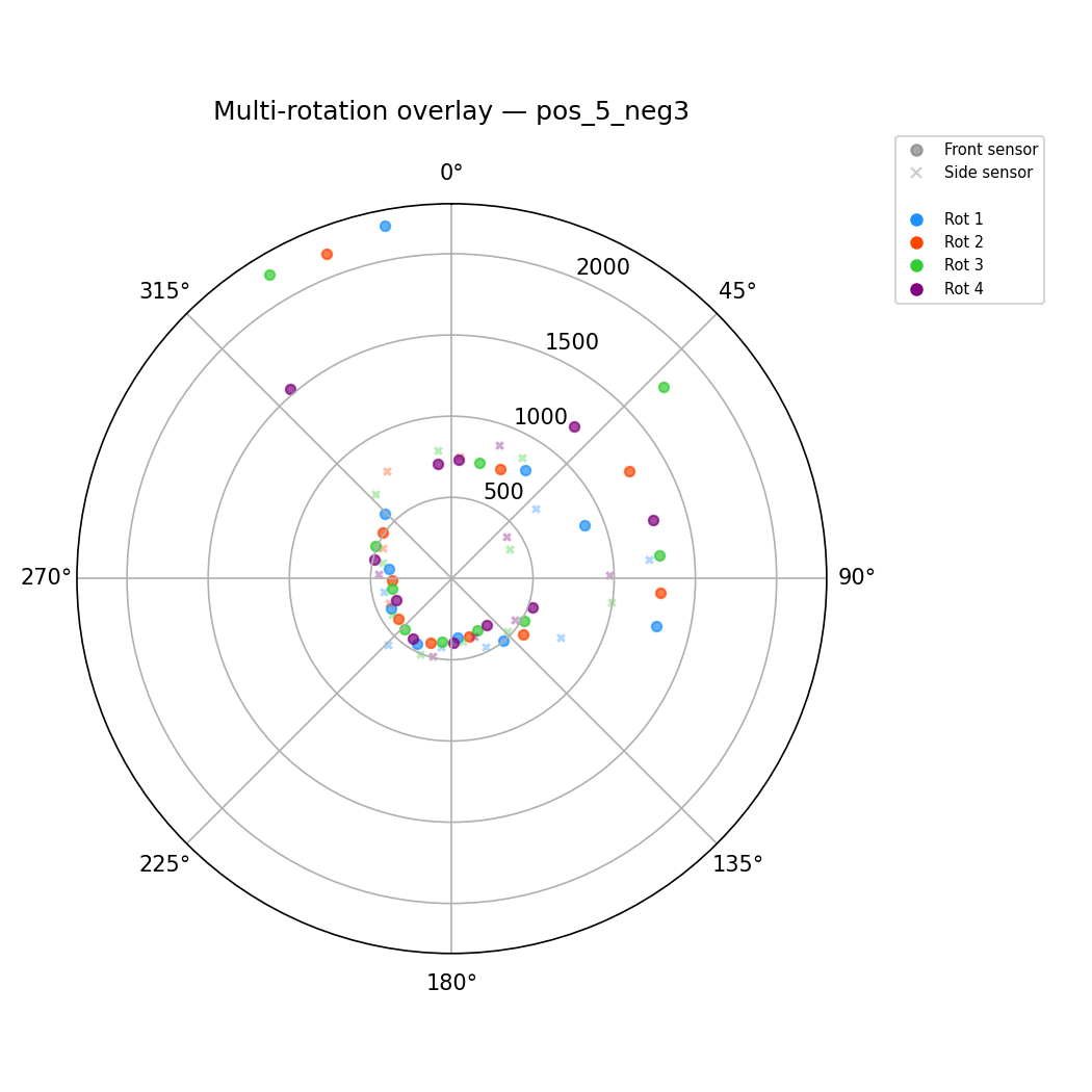
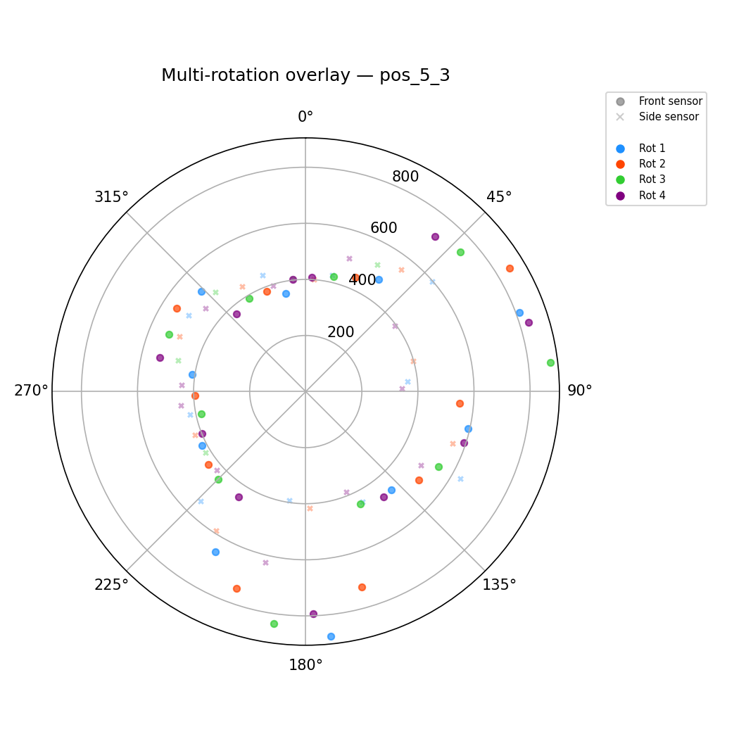
I chose orientation control (PID on integrated gyroscope yaw) for the mapping scan, reusing the PID tuning from Lab 6 (Kp = 8, Kd = 0.52). The robot performs incremental on-axis turns of 35°, stopping at each step to take a stationary ToF reading. Since 35 does not divide 360 evenly (GCD = 5), readings from successive rotations land at different angular positions. Over 41 readings (~4 full rotations), this produces 41 unique angles mod 360° with an average spacing of ~8.8° - well above the lab's minimum of ~25°.

The entire scan is executed autonomously on the Artemis via a state machine (mapping.cpp) that cycles through TURNING → SETTLING (500ms) → READING for each increment. Stopping before each ToF measurement ensures the sensor points at a fixed direction, avoiding the false readings that occur when distance changes during a measurement.

BLE Commands

Two new BLE commands were added for this lab:

On the Python side, a run_scan() helper sets gains, triggers the scan, waits for completion, and retrieves data. Each location's data is saved as JSON for offline replotting.

angles, tof1, tof2 = run_scan(ble, increment=35, num_readings=41,
                                kp=8.0, ki=0.0, kd=0.52)

Orientation Control

PID Performance

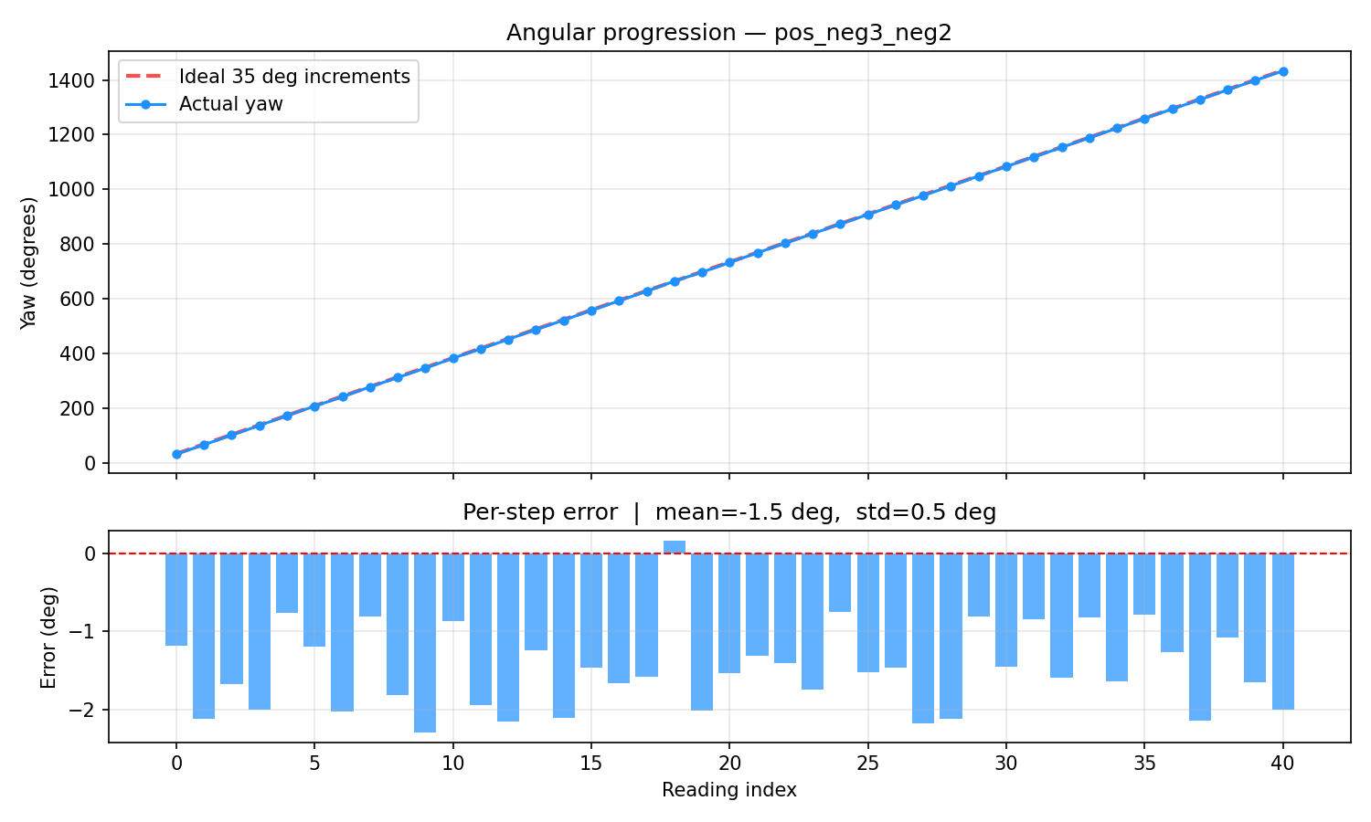
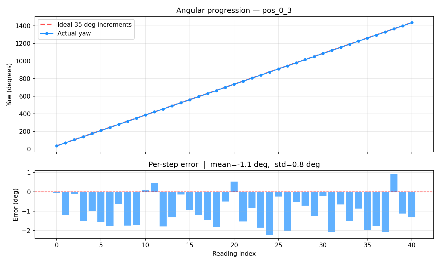
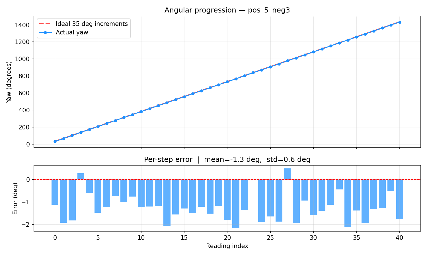
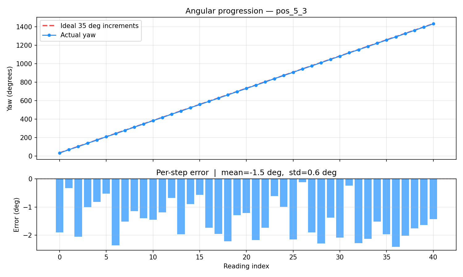
The yaw check plots below compare actual gyro yaw against ideal 35° increments across all 41 readings. The error subplot shows per-step deviation. Across all scan locations, the PID achieves a mean error of ~1.3° with σ < 1°, consistent over 4 full rotations. The small negative bias (~-1.35°) is expected - the 2.5° brake zone in the PID causes the robot to stop just short of each target.

On-Axis Turn Video

I did not realize a video was required until writing this report, so this was recorded on a table at home rather than in the lab. The robot turns roughly on-axis with some visible drift. In the lab, the robot stayed within the 1ft × 1ft grid tiles with less drift - likely due to different surface friction and battery charge. The primary mapping error source is this on-axis drift, as the gyroscope yaw and stationary ToF readings are both very accurate.

Scan Results

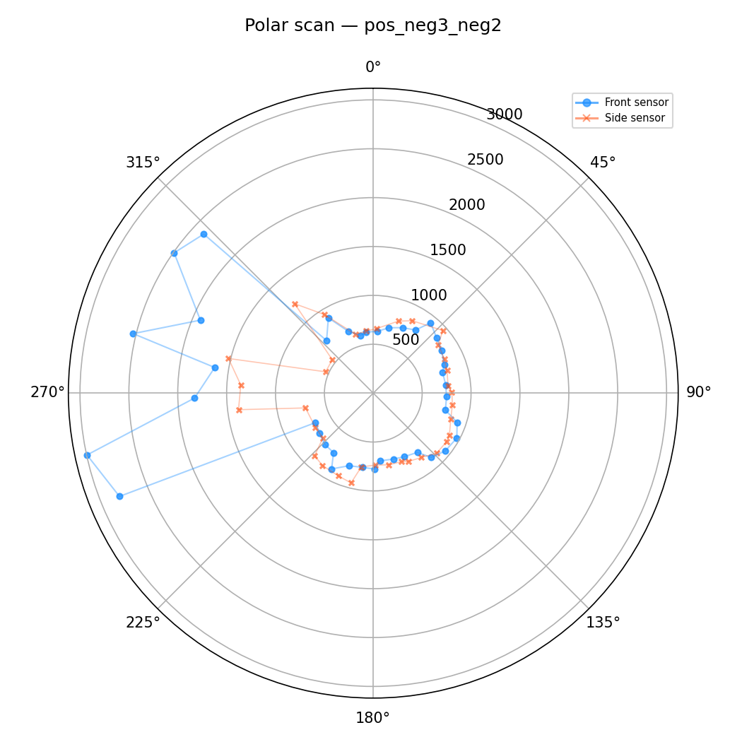
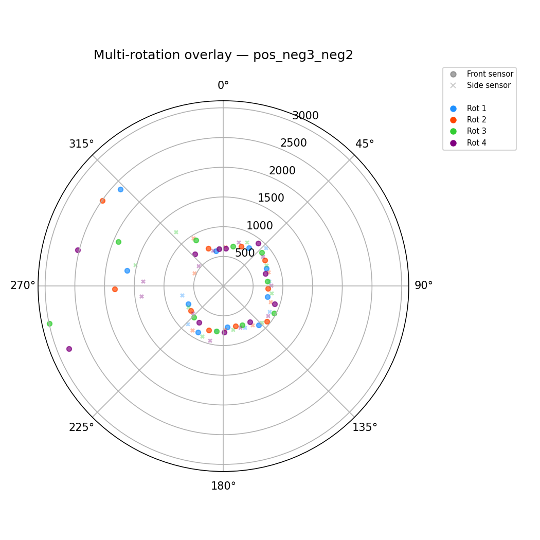
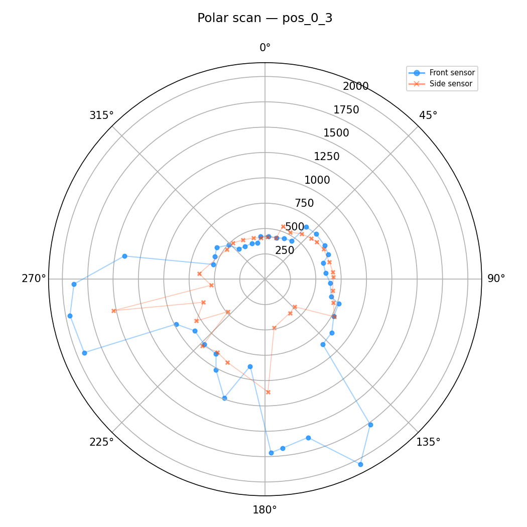
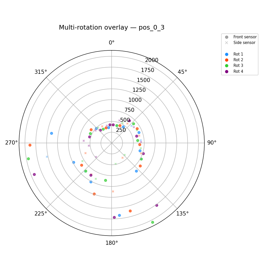
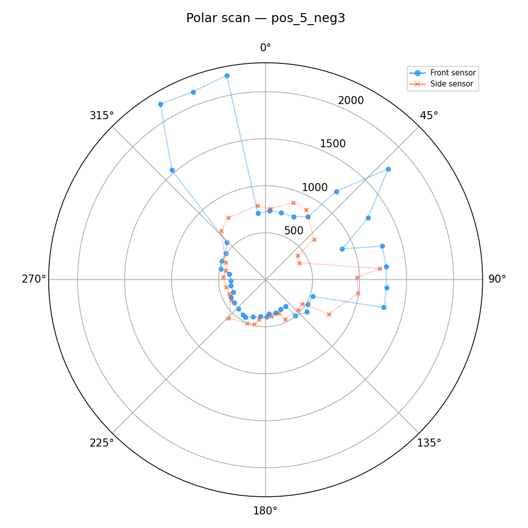
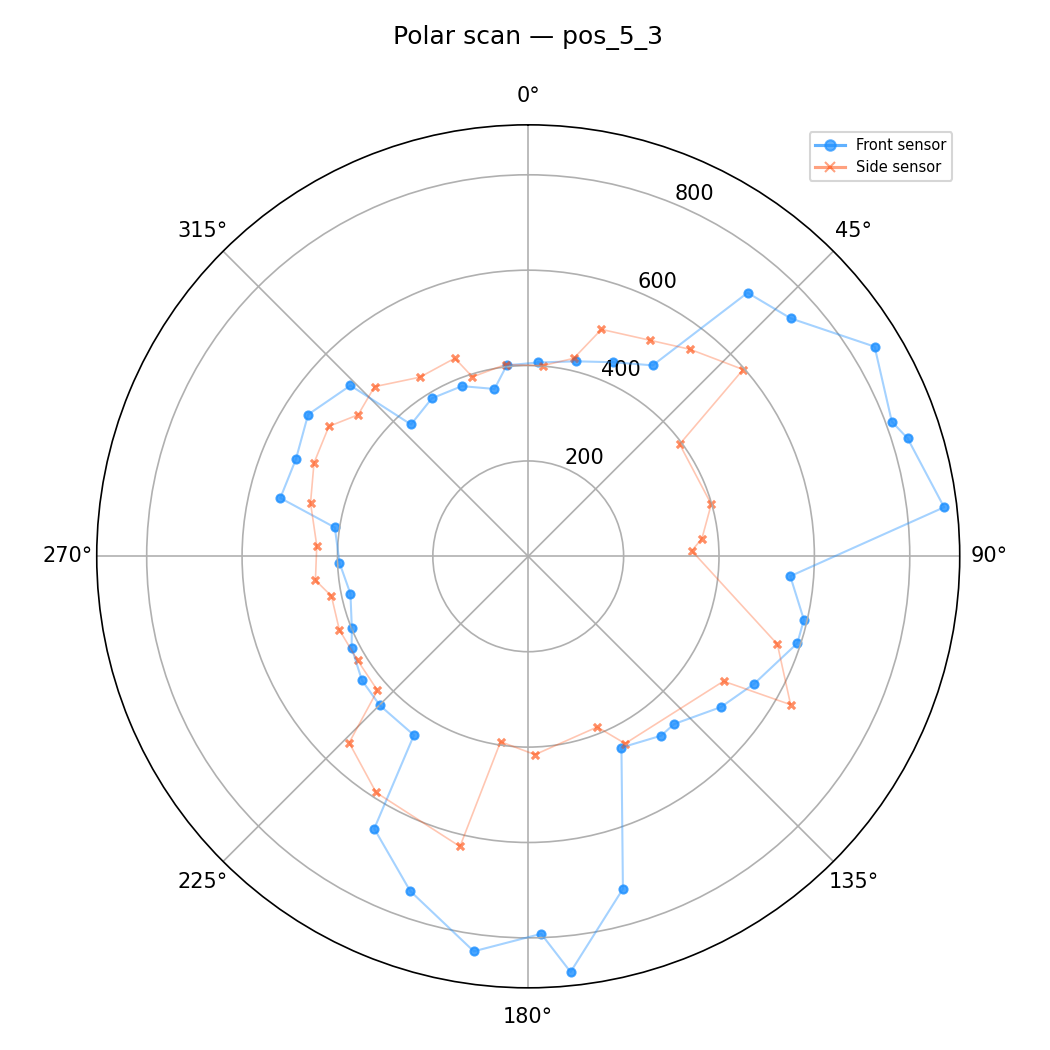
Scans were collected at four marked locations, all with the same starting orientation (front sensor toward +y).

Point 1: (-3, -2)

Point 2: (0, 3)

Point 3: (5, -3)

Point 4: (5, 3)

Merge & Transform

Transformation Matrices

Converting sensor measurements to world coordinates requires two chained transformations.

T1 - Sensor frame → Robot frame. The front ToF sensor is offset ~0.0635 ft (¾ inch) from the robot's center of rotation along its forward axis:

T2 - Robot frame → World (inertial) frame. The robot is at known position $(x_r, y_r)$, rotated by $\theta$ (gyro yaw + initial heading $\theta_0 = 90°$ since the robot starts facing +y):

For a ToF measurement of distance $d$, the sensor-frame point vector is:

The world-frame coordinates are then computed by chaining the transforms:

Which expands to the closed-form equations used in my Python code:

for i in range(len(angles_radians)):
    angle = angles_radians[i]
    d = tof_mm[i] * 0.00328084  # mm to ft

    # T2: robot frame -> world frame
    T_i = np.array([[np.cos(angle), -np.sin(angle), 0, x_r],
                     [np.sin(angle),  np.cos(angle), 0, y_r],
                     [0, 0, 1, 0],
                     [0, 0, 0, 1]])

    # T1: sensor frame -> robot frame
    T_r = np.array([[1, 0, 0, 0.0635],
                     [0, 1, 0, 0],
                     [0, 0, 1, 0],
                     [0, 0, 0, 1]])

    p_tof = np.array([[d], [0], [0], [1]])

    coords = np.matmul(T_i, np.matmul(T_r, p_tof))
    x_coords.append(coords[0][0])
    y_coords.append(coords[1][0])

Since the ToF offset (0.0635 ft ≈ 19mm) is small relative to wall distances, the simplified form x = x_r + d·cos(θ₀ + α) produces nearly identical results.

Merged Plot

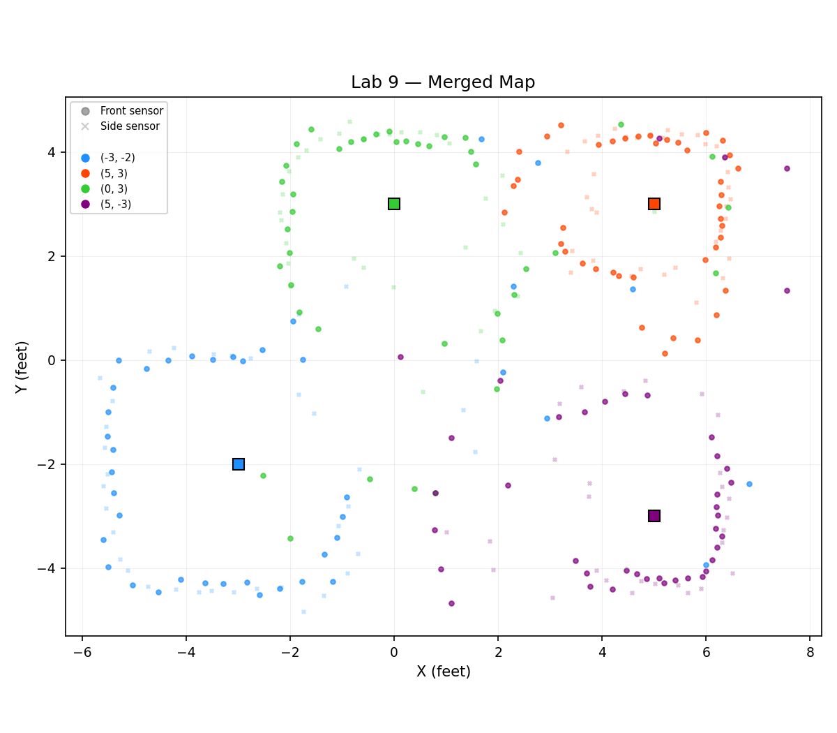
All scans merged into world-frame coordinates. Circles = front sensor, × = side sensor (offset 90°), squares = robot positions.

Line-Based Map

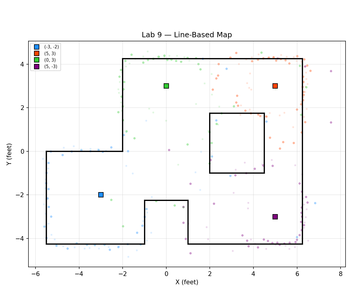
Wall segments were manually estimated from the merged scatter plot. The outer boundary, a left-side notch, a bottom bump, and an interior box obstacle were traced. Wall endpoint lists are saved to line_map.json for Lab 10's simulator.

Error Analysis

For an on-axis turn in the center of a 4×4m empty room (2m to each wall):

Angular error: With a measured mean of ~1.3° and max of ~2.5°, positional error at 2m is 2000mm × sin(1.3°) ≈ 45mm average, and 2000mm × sin(2.5°) ≈ 87mm maximum.

ToF noise: From Lab 3, ±3-11mm depending on range. At 2m, ~11mm. Combined via RSS: √(45² + 11²) ≈ 46mm total error at 2m (~1.5 inches).

Acknowledgements

Claude AI was used for assistance with the mapping state machine implementation, BLE command design, transformation matrix code, plotting utilities, and structuring this lab report. All hardware testing, data collection, PID tuning, scan execution, and wall segment estimation were done by me.